Gaussian blur

The effects of a small and a large Gaussian blur

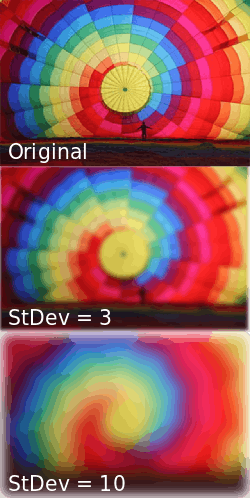
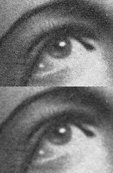
In image processing, a Gaussian blur (also known as Gaussian smoothing) is the result of blurring an image by a Gaussian function. It is a widely used effect in graphics software, typically to reduce image noise and reduce detail. The visual effect of this blurring technique is a smooth blur resembling that of viewing the image through a translucent screen, distinctly different from the bokeh effect produced by an out-of-focus lens or the shadow of an object under usual illumination. Gaussian smoothing is also used as a pre-processing stage in computer vision algorithms in order to enhance image structures at different scales—see scale space representation and scale space implementation.

Mathematically, applying a Gaussian blur to an image is the same as convolving the image with a Gaussian function. This is also known as a two-dimensional Weierstrass transform. By contrast, convolving by a circle (i.e., a circular box blur) would more accurately reproduce the bokeh effect. Since the Fourier transform of a Gaussian is another Gaussian, applying a Gaussian blur has the effect of reducing the image's high-frequency components; a Gaussian blur is thus a low pass filter.

Mathematics

Gaussian blur can be used in order to obtain a smooth grayscale digital image of a halftone print

The Gaussian blur is a type of image-blurring filter that uses a Gaussian function (which also expresses the normal distribution in statistics) for calculating the transformation to apply to each pixel in the image. The equation of a Gaussian function in one dimension is

G(x)={\frac {1}{\sqrt {2\pi \sigma ^{2}}}}e^{-{\frac {x^{2}}{2\sigma ^{2}}}}

in two dimensions, it is the product of two such Gaussians, one in each dimension:

G(x,y)={\frac {1}{2\pi \sigma ^{2}}}e^{-{\frac {x^{2}+y^{2}}{2\sigma ^{2}}}}

^[1]^[2]

Gaussian blurring process: here Gaussian blurring is used to convert a high resolution X-ray image to a low resolution THz image.^[3]

where x is the distance from the origin in the horizontal axis, y is the distance from the origin in the vertical axis, and σ is the standard deviation of the Gaussian distribution. When applied in two dimensions, this formula produces a surface whose contours are concentric circles with a Gaussian distribution from the center point. Values from this distribution are used to build a convolution matrix which is applied to the original image. This convolution process is illustrated visually in the figure on the right. Each pixel's new value is set to a weighted average of that pixel's neighborhood. The original pixel's value receives the heaviest weight (having the highest Gaussian value) and neighboring pixels receive smaller weights as their distance to the original pixel increases. This results in a blur that preserves boundaries and edges better than other, more uniform blurring filters; see also scale space implementation.

In theory, the Gaussian function at every point on the image will be non-zero, meaning that the entire image would need to be included in the calculations for each pixel. In practice, when computing a discrete approximation of the Gaussian function, pixels at a distance of more than 3σ are small enough to be considered effectively zero. Thus contributions from pixels outside that range can be ignored. Typically, an image processing program need only calculate a matrix with dimensions $\lceil 6\sigma \rceil$ × $\lceil 6\sigma \rceil$ (where $\lceil \cdot \rceil$ is the ceiling function) to ensure a result sufficiently close to that obtained by the entire Gaussian distribution.

In addition to being circularly symmetric, the Gaussian blur can be applied to a two-dimensional image as two independent one-dimensional calculations, and so is termed separable filter. That is, the effect of applying the two-dimensional matrix can also be achieved by applying a series of single-dimensional Gaussian matrices in the horizontal direction, then repeating the process in the vertical direction. In computational terms, this is a useful property, since the calculation can be performed in $O\left(w_{\text{kernel}}w_{\text{image}}h_{\text{image}}\right)+O\left(h_{\text{kernel}}w_{\text{image}}h_{\text{image}}\right)$ time (where h is height and w is width; see Big O notation), as opposed to $O\left(w_{\text{kernel}}h_{\text{kernel}}w_{\text{image}}h_{\text{image}}\right)$ for a non-separable kernel.

Applying multiple, successive gaussian blurs to an image has the same effect as applying a single, larger gaussian blur, whose radius is the square root of the sum of the squares of the blur radii that were actually applied. For example, applying successive gaussian blurs with radii of 6 and 8 gives the same results as applying a single gaussian blur of radius 10, since ${\sqrt {6^{2}+8^{2}}}=10$ . Because of this relationship, processing time cannot be saved by simulating a gaussian blur with successive, smaller blurs — the time required will be at least as great as performing the single large blur.

Two downscaled images of the Flag of the Commonwealth of Nations. Before downscaling, a Gaussian blur was applied to the bottom image but not to the top image. The blur makes the image less sharp, but prevents the formation of moiré pattern aliasing artifacts.

Gaussian blurring is commonly used when reducing the size of an image. When downsampling an image, it is common to apply a low-pass filter to the image prior to resampling. This is to ensure that spurious high-frequency information does not appear in the downsampled image (aliasing). Gaussian blurs have nice properties, such as having no sharp edges, and thus do not introduce ringing into the filtered image.

Low-pass filter

Gaussian blur is a low-pass filter, attenuating high frequency signals.

Its amplitude Bode plot (the log scale in the frequency domain) is a parabola.

Variance reduction

How much does a Gaussian filter with standard deviation $\sigma _{f}$ smooth the picture? In other words, how much does it reduce the standard deviation of pixel values in the picture? Assume the grayscale pixel values have a standard deviation $\sigma _{X}$ , then after applying the filter the reduced standard deviation $\sigma _{r}$ can be approximated as

\sigma _{r}\approx {\frac {\sigma _{X}}{\sigma _{f}2{\sqrt {\pi }}}}

Sample Gaussian matrix

This is a sample matrix, produced by sampling the Gaussian filter kernel (with σ = 0.84089642) at the midpoints of each pixel and then normalizing. Note that the center element (at [0, 0]) has the largest value, decreasing symmetrically as distance from the center increases.

0.00000067	0.00002292	0.00019117	0.00038771	0.00019117	0.00002292	0.00000067
0.00002292	0.00078634	0.00655965	0.01330373	0.00655965	0.00078633	0.00002292
0.00019117	0.00655965	0.05472157	0.11098164	0.05472157	0.00655965	0.00019117
0.00038771	0.01330373	0.11098164	0.22508352	0.11098164	0.01330373	0.00038771
0.00019117	0.00655965	0.05472157	0.11098164	0.05472157	0.00655965	0.00019117
0.00002292	0.00078633	0.00655965	0.01330373	0.00655965	0.00078633	0.00002292
0.00000067	0.00002292	0.00019117	0.00038771	0.00019117	0.00002292	0.00000067

Note that 0.22508352 (the central one) is 1177 times larger than 0.00019117 which is just outside 3σ.

Implementation

A Gaussian blur effect is typically generated by convolving an image with a kernel of Gaussian values. In practice, it is best to take advantage of the Gaussian blur’s separable property by dividing the process into two passes. In the first pass, a one-dimensional kernel is used to blur the image in only the horizontal or vertical direction. In the second pass, the same one-dimensional kernel is used to blur in the remaining direction. The resulting effect is the same as convolving with a two-dimensional kernel in a single pass, but requires fewer calculations.

Discretisation is typically achieved by sampling the Gaussian filter kernel at discrete points, normally at positions corresponding to the midpoints of each pixel. This reduces the computational cost but, for very small filter kernels, point sampling the Gaussian function with very few samples leads to a large error. In these cases, accuracy is maintained (at a slight computational cost) by integration of the Gaussian function over each pixel's area.^[4]

When converting the Gaussian’s continuous values into the discrete values needed for a kernel, the sum of the values will be different from 1. This will cause a darkening or brightening of the image. To remedy this, the values can be normalized by dividing each term in the kernel by the sum of all terms in the kernel.

Common uses

This shows how smoothing affects edge detection. With more smoothing, fewer edges are detected

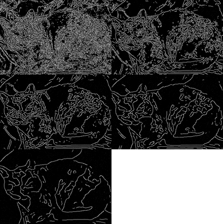
Gaussian smoothing is commonly used with edge detection. Most edge-detection algorithms are sensitive to noise; the 2-D Laplacian filter, built from a discretization of the Laplace operator, is highly sensitive to noisy environments. Using a Gaussian Blur filter before edge detection aims to reduce the level of noise in the image, which improves the result of the following edge-detection algorithm. This approach is commonly referred to as Laplacian of Gaussian, or LoG filtering.^[5]

Notes and references

↑ Shapiro, L. G. & Stockman, G. C: "Computer Vision", page 137, 150. Prentice Hall, 2001
↑ Mark S. Nixon and Alberto S. Aguado. Feature Extraction and Image Processing. Academic Press, 2008, p. 88.
↑ Ahi, Kiarash (May 26, 2016). "Modeling of terahertz images based on x-ray images: a novel approach for verification of terahertz images and identification of objects with fine details beyond terahertz resolution". Proc. SPIE 9856, Terahertz Physics, Devices, and Systems X: Advanced Applications in Industry and Defense, 985610. doi:10.1117/12.2228685. Retrieved May 26, 2016.
↑ Erik Reinhard. High dynamic range imaging: Acquisition, Display, and Image-Based Lighting. Morgan Kaufmann, 2006, pp. 233–234.
↑ Fisher, Perkins, Walker & Wolfart (2003). "Spatial Filters - Laplacian of Gaussian". Retrieved 2010-09-13.

External links

GLSL implementation of a separable gaussian blur filter.
Example for Gaussian blur (low pass filtering) applied to a wood-block print and an etching in order to remove details for picture comparison.
Mathematica GaussianFilter function

This article is issued from Wikipedia - version of the 9/14/2016. The text is available under the Creative Commons Attribution/Share Alike but additional terms may apply for the media files.