Gradient-Enhanced Kriging (GEK)

Gradient-Enhanced Kriging (GEK) is a surrogate modeling technique used in engineering. A surrogate model (alternatively known as a metamodel, response surface or emulator) is a prediction of the output of an expensive computer code. This prediction is based on a small number of evaluations of the expensive computer code.

Introduction

Example of one-dimensional data interpolated by Kriging and GEK. The black line indicates the test-function, while the gray circles indicate 'observations', 'samples' or 'evaluations' of the test-function. The blue line is the Kriging mean, the shaded blue area illustrates the Kriging standard deviation. With GEK we can add the gradient information, illustrated in red, which increases the accuracy of the prediction.

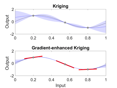
Adjoint solvers are now becoming available in a range of Computational Fluid Dynamics (CFD) solvers, such as Fluent, OpenFOAM, SU2 and US3D. Originally developed for optimization, adjoint solvers are now finding more and more use in uncertainty quantification.

Linear speedup

An adjoint solver allows one to compute the gradient of the quantity of interest with respect to all design parameters at the cost of one additional solve. This, potentially, leads to a linear speedup: the computational cost of constructing an accurate surrogate decrease, and the resulting computational speedup $s$ scales linearly with the number $d$ of design parameters.

The reasoning behind this linear speedup is straightforward. Assume we run $N$ primal solves and $N$ adjoint solves, at a total cost of $2N$. This results in ${\displaystyle N+dN}$ data; $N$ values for the quantity of interest and $d$ partial derivatives in each of the $N$ gradients. Now assume that each partial derivative provides as much information for our surrogate as a single primal solve. Then, the total cost of getting the same amount of information from primal solves only is ${\displaystyle N+dN}$. The speedup is the ratio of these costs: ^{[1] [2]}

${\displaystyle s={\frac {N+dN}{2N}}={\frac {1}{2}}+{\frac {1}{2}}d}$.

A linear speedup has been demonstrated for a fluid-structure interaction problem ^[1] and for a transonic airfoil.^[2]

Noise

One issue with adjoint-based gradients in CFD is that they can be particularly noisy. ^{[3] [4]} When derived in a Bayesian framework, GEK allows one to incorporate not only the gradient information, but also the uncertainty in that gradient information.^[5]

Approach

When using GEK one takes the following steps:

1. Create a Design of Experiment (DoE): The DoE or 'sampling plan' is a list of different locations in the design space. The DoE indicates which combinations of parameters one will use to sample the computer simulation. With Kriging and GEK, a common choice is to use a Latin Hypercube Design (LHS) design with a 'maximin' criterion. The LHS-design is available in scripting codes like MATLAB or Python.
2. Make observations: For each sample in our DoE one runs the computer simulation to obtain the Quantity of Interest (QoI).
3. Construct the surrogate: One uses the GEK predictor equations to construct the surrogate conditional on the obtained observations.

Once the surrogate has been constructed it can be used in different ways, for example for surrogate-based Uncertainty Quantification (UQ) or optimization.

Predictor equations

In a Bayesian framework, we use Bayes' Theorem to predict the Kriging mean and covariance conditional on the observations. When using GEK, the observations are usually the results of a number of computer simulations. GEK can be interpreted as a form of Gaussian process regression.

Kriging

Along the lines of ^{[5] [6]} , we are interested in the output $x$ of our computer simulation, for which we assume the normal prior probability distribution:

${\displaystyle x\sim {\mathcal {N}}(\mu ,P)}$,

with prior mean $\mu$ and prior covariance matrix $P$. The observations $y$ have the normal likelihood:

${\displaystyle y|x\sim {\mathcal {N}}(Hx,R)}$,

with $H$ the observation matrix and $R$ the observation error covariance matrix, which contains the observation uncertainties. After applying Bayes' Theorem we obtain a normally distributed posterior probability distribution, with Kriging mean:

${\displaystyle \mathrm {E} (x|y)=\mu +K(y-H\mu )}$,

and Kriging covariance:

${\displaystyle \mathrm {cov} (x|y)=(I-KH)P}$,

where we have the gain matrix:

${\displaystyle K=PH^{T}(R+HPH^{T})^{-1}}$.

In Kriging, the prior covariance matrix $P$ is generated from a covariance function. One example of a covariance function is the Gaussian covariance:

${\displaystyle P_{ij}=\sigma ^{2}\mathrm {exp} \left(-\sum _{k}{\frac {|x_{jk}-x_{ik}|^{2}}{2\theta _{k}^{2}}}\right)}$,

where we sum over the dimensions $k$. The hyperparameters $\mu$, $\sigma$ and $\theta$ can be estimated from a Maximum Likelihood Estimate (MLE).^[5]

Indirect GEK

There are several ways of implementing GEK. The first method, indirect GEK, defines a small but finite stepsize $h$, and uses the gradient information to append synthetic data to the observations $y$, see for example.^[7] Indirect Kriging is sensitive to the choice of the stepsize $h$ and cannot include observation uncertainties.

Direct GEK (through prior covariance matrix)

Direct GEK is a form of co-Kriging, where we add the gradient information as co-variables. This can be done by modifying the prior covariance $P$ or by modifying the observation matrix $H$; both approaches lead to the same GEK predictor. When we construct direct GEK through the prior covariance matrix, we append the partial derivatives to $y$, and modify the prior covariance matrix $P$ such that it also contains the derivatives (and second derivatives) of the covariance function, see for example ^[5] .^[8] The main advantages of direct GEK over indirect GEK are: 1) we do not have to choose a stepsize, 2) we can include observation uncertainties for the gradients in $R$, and 3) it is less susceptible to poor conditioning of the gain matrix $K$. ^{[5] [7]}

Direct GEK (through observation matrix)

Another way of arriving at the same direct GEK predictor is to append the partial derivatives to the observations $y$ and include partial derivative operators in the observation matrix $H$, see for example ^[9] .

Example: Drag coefficient of a transonic airfoil

Transonic airfoil.

Reference results for the drag coefficient of a transonic airfoil, based on a large number of CFD simulations. The horizontal and vertical axis show the deformation of the shape of the airfoil.

Kriging surrogate model of the drag coefficient of a transonic airfoil. The gray dots indicate the configurations for which the CFD solver was run.

GEK surrogate model of the drag coefficient of a transonic airfoil. The gray dots indicate the configurations for which the CFD solver was run, the arrows indicate the gradients.

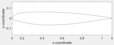
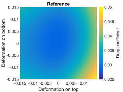
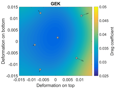
As an example, let us consider the flow over a transonic airfoil.^[2] The airfoil is operating at a Mach number of 0.8 and an angle of attack of 1.25 degrees. We assume that the shape of the airfoil is uncertain; the top and the bottom of the airfoil might have shifted up or down due to manufacturing tolerances. In other words, the shape of the airfoil that we are using might be slightly different from the airfoil that we designed.

On the right we see the reference results for the drag coefficient of the airfoil, based on a large number of CFD simulations. Note that the lowest drag, which corresponds to 'optimal' performance, is close to the undeformed 'baseline' design of the airfoil at (0,0).

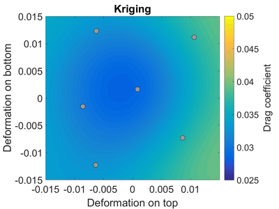
After designing a sampling plan (indicated by the gray dots) and running the CFD solver at those sample locations, we obtain the Kriging surrogate model. The Kriging surrogate is close to the reference, but perhaps not as close as we would desire.

In the last figure, we have improved the accuracy of this surrogate model by including the adjoint-based gradient information, indicated by the arrows, and applying GEK.

Applications

GEK has found the following applications:

• 1993: Design problem for a borehole model test-function.^[10]
• 2002: Aerodynamic design of a supersonic business jet.^[11]
• 2008: Uncertainty quantification for a transonic airfoil with uncertain shape parameters.^[8]
• 2009: Uncertainty quantification for a transonic airfoil with uncertain shape parameters.^[7]
• 2012: Surrogate model construction for a panel divergence problem, a fluid-structure interaction problem. Demonstration of a linear speedup.^[1]
• 2014: Uncertainty quantification for the RANS simulation of an airfoil, with the model parameters of the k-epsilon turbulence model as uncertain inputs.^[5]
• 2015: Uncertainty quantification for the Euler simulation of a transonic airfoil with uncertain shape parameters. Demonstration of a linear speedup.^[2]
• 2016: Surrogate model construction for two fluid-structure interaction problems.^[12]

References

1. de Baar, J.H.S.; Scholcz, T.P.; Verhoosel, C.V.; Dwight, R.P.; van Zuijlen, A.H.; Bijl, H. (2012). "Efficient uncertainty quantification with gradient-enhanced Kriging: Applications in FSI" (PDF). ECCOMAS, Vienna, Austria, September 10–14.
2. de Baar, J.H.S.; Scholcz, T.P.; Dwight, R.P. (2015). "Exploiting Adjoint Derivatives in High-Dimensional Metamodels". AIAA Journal. 53 (5): 1391–1395.
3. Dwight, R.; Brezillon, J. (2006). "Effect of Approximations of the Discrete Adjoint on Gradient-Based Optimization". AIAA Journal. 44 (12): 3022–3031.
4. Giles, M.; Duta, M.; Muller, J.; Pierce, N. (2003). "Algorithm Developments for Discrete Adjoint Methods". AIAA Journal. 41 (2): 198–205.
5. de Baar, J.H.S.; Dwight, R.P.; Bijl, H. (2014). "Improvements to gradient-enhanced Kriging using a Bayesian interpretation". International Journal for Uncertainty Quantification. 4 (3): 205–223.
6. Wikle, C.K.; Berliner, L.M. (2007). "A Bayesian tutorial for data assimilation". Phys. D: Nonlin. Phenom. 230 (1-2): 1–16.
7. Dwight, R.P.; Han, Z.-H. (2009). "Efficient uncertainty quantification using gradient-enhanced Kriging". 11th AIAA Non-Deterministic Approaches Conference, Palm Springs, California, 4–7 May.
8. Laurenceau, J.; Sagaut, P. (2008). "Building efficient response surfaces of aerodynamic functions with Kriging and coKriging". AIAA Journal. 46 (2): 498–507.
9. de Baar, J.H.S. (2014). Stochastic Surrogates for Measurements and Computer Models of Fluids. PhD thesis, Delft University of Technology. pp. 99–101.
10. Morris, M.D.; Mitchell, T.J.; Ylvisaker, D. (1993). "Bayesian Design and Analysis of Computer Experiments: Use of Derivatives in Surface Prediction". Technometrics. 35 (3): 243–255.
11. Chung, H.-S.; Alonso, J.J. (2002). "Using Gradients to Construct Cokriging Approximation Models for High-Dimensional Design Optimization Problems". AIAA 40th Aerospace Sciences Meeting and Exhibit.
12. Ulaganathan, S.; Couckuyt, I.; Dhaene, T.; Degroote, J.; Laermans, E. (2016). "Performance study of gradient-enhanced Kriging". Engineering with Computers. 32 (1): 15–34.