Leapfrog filter

A low-pass ladder filter and its signal flow graph

A leapfrog filter is a type of active circuit electronic filter that simulates a passive electronic ladder filter. Other names for this type of filter are active-ladder or multiple feedback filter.^[1]:286 The arrangement of feedback loops in the signal flow-graph of the simulated ladder filter inspired the name leapfrog filter.^[1]:286 The leapfrog filter maintains the low component sensitivity of the passive ladder filter that it simulates. ^{[lower-alpha 1]:291}

Synthesis

Generic ladder filters with either (a) voltage input/voltage output, (b) current input/voltage output, (c) voltage input/current output or (d) current input/ current output. The output may also be the voltage across or the current through an internal component of the last element.

The definition and synthesis of leapfrog filters is described by Temes & LaPatra,^{[1]:281–291} Chen^[2] and Wait, Huelsman & Korn.^[3]

Synthesis of leapfrog filters typically includes the following steps:

1. Determine a prototype passive ladder filter that has the desired frequency response. Usually a doubly terminated prototype is used.

2. Write the equations relating element current to voltage across the element in a form suitable for expression as a signal-flow graph.

3. Draw the signal-flow graph. The nodes of the signal-flow graph will include both voltages and currents. The branch gains will include impedances and admittances.

4. Convert all nodes of the signal-flow graph to voltages and all impedances to dimensionless transmittances. This is accomplished by dividing all impedance elements by R, an arbitrary resistance and multiplying all admittance elements by R. This scaling does not change the frequency response.

5. Manipulate the signal-flow graph so that the gains feeding each summing node have the same signs. This is done as an implementation convenience. At the completion of this step, typically, all the feedback gains in the signal-flow graph will be +1 and the signs of the gain blocks in the forward path will alternate. As a result, some of the nodes, including the main output, may have a 180° phase inversion. This is usually of no consequence.^[2]:2445

6. The gain blocks are implemented with active filters and interconnected as indicated by the signal-flow graph. Often, state variable filters are used for the gain blocks.

7. The final circuit usually has more components than the prototype passive filter. This means the final circuit has degrees of freedom which can be chosen to optimize the circuit for dynamic range^[2]:2449 and for practical component values.

Examples

Generic filter

Four element ladder filter with voltage input and voltage output

Three stages of signal-flow graph development of a four element ladder filter with voltage input and voltage output.

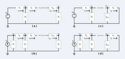
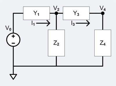
The design starts out with a known ladder filter of one of the typologies shown in the previous figure. Usually, all the elements of the ladder filter are lossless except the first and the last which are lossy.^[2]:2442 Using a four element voltage input, voltage output ladder filter^{[lower-alpha 2]} as an example, the equations that relate the element voltages and currents are as follows:

${\displaystyle I_{1}=(V_{0}-V_{2})\mathrm {Y_{1}} }$

${\displaystyle V_{2}=(I_{1}-I_{3})\mathrm {Z_{2}} }$

${\displaystyle I_{3}=(V_{2}-V_{4})\mathrm {Y_{3}} }$

${\displaystyle V_{4}=(I_{3})\mathrm {Z_{4}} }$

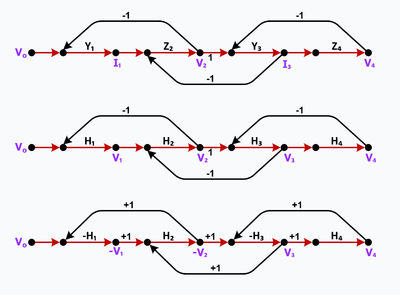
The signal-flow graph for these equations are shown in the second figure to the right. The arrangement of feedback loops in the signal flow-graph inspired the name leapfrog filter.^[1]:286 The signal flow graph is manipulated to convert all current nodes into voltage nodes and all the impedances and admittances into dimensionless transmittances. This is equivalent to manipulating the equations either by multiplying both sides by R or by multiplying one side by R/R and distributing the R terms across the subtraction operation. This manipulation changes the equations as follows:

${\displaystyle V_{1}=(V_{0}-V_{2})\mathrm {H_{1}} }$

${\displaystyle V_{2}=(V_{1}-V_{3})\mathrm {H_{2}} }$

${\displaystyle V_{3}=(V_{2}-V_{4})\mathrm {H_{3}} }$

${\displaystyle V_{4}=(V_{3})\mathrm {H_{4}} }$

where H₁ = RY₁, H₂ = GZ₂, H₃ = RY₃, H₄ = GZ₄, G = 1/R, V₁ = RI₁, V₃ = RI₃

The signal flow graph is further manipulated so that the gains into each summing node is +1. The result of all the manipulation is shown as the bottom signal-flow graph in the figure. The equations represented by the resulting signal flow graph are as follows:

${\displaystyle -V_{1}=(V_{0}-V_{2})(-\mathrm {H_{1}} )}$

${\displaystyle -V_{2}=(-V_{1}+V_{3})\mathrm {H_{2}} }$

${\displaystyle V_{3}=(-V_{2}+V_{4})(-\mathrm {H_{3}} )}$

${\displaystyle V_{4}=(V_{3})\mathrm {H_{4}} }$

The awkward annotation of -V₁ and -V₂ as labels of nodes in the signal flow graph indicates that these nodes present a 180° phase inversion with respect to the signals in the prototype filter.

This manipulation is can be accomplished by a simple procedure:

1. Make all the odd numbered or all the even numbered transmittances negative. The overall phase shift with respect to the prototype will be 0° if the total number of inversions is even.

2. Change all feedback gains to +1.

3. Determine the sign of each node label by counting the number of inversions to that node from the input. If the number of inversions is odd, then the node label is negative.

The signal-flow graph is suitable for implementation. State variable filters that are available in both inverting and non-inverting typologies are often used.

Band pass filter

A schematic for a passive band pass electronic filter

Passive circuit

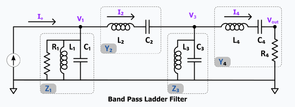
The circuit for a band pass, passive ladder filter is first determined.

The individual components in parallel or series can be combined into general impedances or admittances. For this schematic:

${\displaystyle \mathrm {Z_{1}} ={\frac {s\mathrm {L_{1}} }{s^{2}\mathrm {C_{1}} \mathrm {L_{1}} +s{\frac {\mathrm {L_{1}} }{\mathrm {R_{1}} }}+\mathrm {1} }}}$

${\displaystyle {\mathrm {Y_{2}} }={\frac {s\mathrm {C_{2}} }{s^{2}\mathrm {C_{2}} \mathrm {L_{2}} +\mathrm {1} }}}$

${\displaystyle \mathrm {Z_{3}} ={\frac {s\mathrm {L_{3}} }{s^{2}\mathrm {C_{3}} \mathrm {L_{3}} +1}}}$

${\displaystyle \mathrm {Y_{4}} ={\frac {s\mathrm {C_{4}} }{s^{2}\mathrm {C_{4}} \mathrm {L_{4}} +s\mathrm {C_{4}} \mathrm {R_{4}} +1}}}$

The signal flow-graph representation of the ladder filter equations.

Signal-flow graph

The current and voltage variables can be put into cause and effect relationships as follows.

$V_{1}=(I_{0}-I_{2}){\mathrm {Z_{1}}}$

${\displaystyle I_{2}=(V_{1}-V_{3})\mathrm {Y_{2}} }$

${\displaystyle V_{3}=(I_{2}-I_{4})\mathrm {Z_{3}} }$

${\displaystyle I_{4}=V_{3}\mathrm {Y_{4}} }$

${\displaystyle V_{4}=I_{4}\mathrm {R_{4}} }$

A signal flow graph for these equations is shown to the right.

Scaled signal-flow graph

For implementation reasons, the current variables may be multiplied by an arbitrary resistance to convert them into voltage variables which also converts all gains to dimensionless values. In this example all currents are multiplied by R. This is accomplished by either multiplying both sides of an equation by R of by multiplying one side by R/R and then distributing the R term over the currents.

The signal flow-graph representation of the ladder filter equations with impedances scaled by R, an arbitrary resistance.

${\displaystyle V_{1}=(V_{0}-V_{2})\mathrm {H_{1}} }$

${\displaystyle V_{2}=(V_{1}-V_{3})\mathrm {H_{2}} }$

${\displaystyle V_{3}=(V_{2}-V_{4})\mathrm {H_{3}} }$

${\displaystyle V_{4}=(V_{3})\mathrm {H_{4}} }$

${\displaystyle V_{\mathrm {out} }=(V_{4})\mathrm {H_{5}} }$

where H₁ = GZ₁, H₂ = RY₂, H₃ = GZ₃, H₄ = RY₄, H₅ = GR₄, G = 1/R, V₂ = RI₂, V₄ = RI₄

Manipulated signal-flow graph

It is convenient for implementation if the gains feeding the summing nodes all have the same sign. In that case, summation can be achieved with a junction of two resisters.

The signal flow-graph representation of the ladder filter equations with impedances scaled by R, an arbitrary resistance. The signs of the gains have been manipulated so that all gains feeding into a node have the same signs.

${\displaystyle V_{1}=(V_{0}+(-V_{2}))\mathrm {H_{1}} }$

${\displaystyle -V_{2}=(V_{1}+(-V_{3}))(\mathrm {-H_{2}} )}$

${\displaystyle -V_{3}=((-V_{2})+V_{4})\mathrm {H_{3}} }$

${\displaystyle V_{4}=V_{3}(\mathrm {-H_{4}} )}$

${\displaystyle V_{\mathrm {out} }=(V_{4})\mathrm {H_{5}} }$

Implementation

Modified Tow-Thomas active biquad filter with summing inputs and complimentary band pass outputs suitable for use in a leapfrog filter. V_BP is the bandpass output, V_BPI is the inverted bandpass output.

All the transmittances H₁ - H₄, in this example, are bandpass filters. They can be implemented with the modified Tow-Thomas active biquad filter. This biquad has both positive and negative bandpass outputs so that it can realize any of the transmittances. This biquad also has summing inputs so it can also implement the summing nodes.^[3]:302

Tuning

A leapfrog filter can be difficult to tune because of the complicated feed back. One strategy is to open the feedback loops so that the remaining filter structure is a simple cascade design. Each section can then be tuned independently. The inner sections, H₂ and H₃ have infinite Q and may be unstable when the feedback loops are opened. These stages may be designed with a large, but finite Q so that they can be tuned while the feedback loops are open.

Notes

1. "Hence, the low sensitivity property of the doubly loaded LC ladder is preserved." ^[1]
2. Based on the circuit shown in Temes & LaPatra figure 7-30 (a) ,^[1]:287

References

1. Temes, Gabor C.; LaPatra, Jack W. (1977). Circuit Synthesis and Design. McGraw-Hill. ISBN 0-07-063489-0.
2. Chen, Wai-Kai (1995). The Circuits and Filters Handbook. CRC Press. pp. 622–638,2442–2459. ISBN 0-8493-8341-2.
3. Wait, John V.; Huelsman, Lawrence P.; Korn, Granino A. (1992). Introduction to Operational Amplifier Theory and Applications (2nd ed.). McGraw-Hill. pp. 295–303. ISBN 0-07-067770-0.