Linear equation

Graph sample of linear equations.

A linear equation is an algebraic equation in which each term is either a constant or the product of a constant and (the first power of) a single variable. A simple example of a linear equation with only one variable, $x$ , may be written in the form: $ax + b = 0$ , where $a$ and $b$ are constants and $a \neq 0$ . The constants may be numbers, parameters, or even non-linear functions of parameters, and the distinction between variables and parameters may depend on the problem (for an example, see linear regression).

Linear equations can have one or more variables. An example of a linear equation with three variables, $x$ , $y$ , and $z$ , is given by: $ax + by + cz + d = 0$ , where $a, b, c$ , and $d$ are constants and $a, b$ , and $c$ are non-zero. Linear equations occur frequently in most subareas of mathematics and especially in applied mathematics. While they arise quite naturally when modeling many phenomena, they are particularly useful since many non-linear equations may be reduced to linear equations by assuming that quantities of interest vary to only a small extent from some "background" state. An equation is linear if the sum of the exponents of the variables of each term is one.

Equations with exponents greater than one are non-linear. An example of a non-linear equation of two variables is $axy + b = 0$ , where $a$ and $b$ are constants and $a \neq 0$ . It has two variables, $x$ and $y$ , and is non-linear because the sum of the exponents of the variables in the first term, $axy$ , is two.

This article considers the case of a single equation for which one searches the real solutions. All its content applies for complex solutions and, more generally for linear equations with coefficients and solutions in any field.

One variable

A linear equation in one unknown $x$ may always be rewritten

ax=b.

If $a \neq 0$ , there is a unique solution

x={\frac {b}{a}}.

If $a = 0$ , then, when $b = 0$ every number is a solution of the equation, but if $b \neq 0$ there are no solutions (and the equation is said to be inconsistent.)

Two variables

A common form of a linear equation in the two variables x and y is

y=mx+b,\,

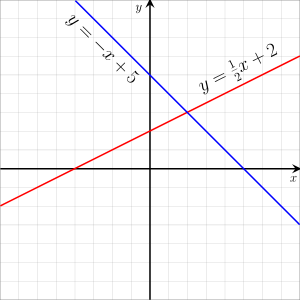
where m and b designate constants (parameters). The origin of the name "linear" comes from the fact that the set of solutions of such an equation forms a straight line in the plane. In this particular equation, the constant m determines the slope or gradient of that line, and the constant term b determines the point at which the line crosses the y-axis, otherwise known as the y-intercept.

Since terms of linear equations cannot contain products of distinct or equal variables, nor any power (other than 1) or other function of a variable, equations involving terms such as xy, x², y^1/3, and sin(x) are nonlinear.

Forms for two-dimensional linear equations

Linear equations can be rewritten using the laws of elementary algebra into several different forms. These equations are often referred to as the "equations of the straight line." In what follows, x, y, t, and θ are variables; other letters represent constants (fixed numbers).

General (or standard) form

In the general (or standard^[1]) form the linear equation is written as:

Ax+By=C,\,

where A and B are not both equal to zero. The equation is usually written so that A ≥ 0, by convention. The graph of the equation is a straight line, and every straight line can be represented by an equation in the above form. If A is nonzero, then the x-intercept, that is, the x-coordinate of the point where the graph crosses the x-axis (where, y is zero), is C/A. If B is nonzero, then the y-intercept, that is the y-coordinate of the point where the graph crosses the y-axis (where x is zero), is C/B, and the slope of the line is −A/B. The general form is sometimes written as:

ax+by+c=0,\,

where a and b are not both equal to zero. The two versions can be converted from one to the other by moving the constant term to the other side of the equal sign.

Slope–intercept form

y=mx+b,

where m is the slope of the line and b is the y intercept, which is the y coordinate of the location where the line crosses the y axis. This can be seen by letting x = 0, which immediately gives y = b. It may be helpful to think about this in terms of y = b + mx; where the line passes through the point (0, b) and extends to the left and right at a slope of m. Vertical lines, having undefined slope, cannot be represented by this form.

Point–slope form

y-y_{1}=m(x-x_{1}),\,

where m is the slope of the line and (x₁,y₁) is any point on the line.

The point-slope form expresses the fact that the difference in the y coordinate between two points on a line (that is, y − y₁) is proportional to the difference in the x coordinate (that is, x − x₁). The proportionality constant is m (the slope of the line).

Two-point form

y-y_{1}={\frac {y_{2}-y_{1}}{x_{2}-x_{1}}}(x-x_{1}),\,

where (x₁, y₁) and (x₂, y₂) are two points on the line with x₂ ≠ x₁. This is equivalent to the point-slope form above, where the slope is explicitly given as (y₂ − y₁)/(x₂ − x₁).

Multiplying both sides of this equation by (x₂ − x₁) yields a form of the line generally referred to as the symmetric form:

(x_{2}-x_{1})(y-y_{1})=(y_{2}-y_{1})(x-x_{1}).\,

Expanding the products and regrouping the terms leads to the general form:

x\,(y_{2}-y_{1})-y\,(x_{2}-x_{1})=x_{1}y_{2}-x_{2}y_{1}

Using a determinant, one gets a determinant form, easy to remember:

{\begin{vmatrix}x&y&1\\x_{1}&y_{1}&1\\x_{2}&y_{2}&1\end{vmatrix}}=0\,.

Intercept form

{\frac {x}{a}}+{\frac {y}{b}}=1,\,

where a and b must be nonzero. The graph of the equation has x-intercept a and y-intercept b. The intercept form is in standard form with A/C = 1/a and B/C = 1/b. Lines that pass through the origin or which are horizontal or vertical violate the nonzero condition on a or b and cannot be represented in this form.

Matrix form

Using the order of the standard form

Ax+By=C,\,

one can rewrite the equation in matrix form:

{\begin{pmatrix}A&B\end{pmatrix}}{\begin{pmatrix}x\\y\end{pmatrix}}={\begin{pmatrix}C\end{pmatrix}}.

Further, this representation extends to systems of linear equations.

A_{1}x+B_{1}y=C_{1},\,

A_{2}x+B_{2}y=C_{2},\,

becomes:

{\begin{pmatrix}A_{1}&B_{1}\\A_{2}&B_{2}\end{pmatrix}}{\begin{pmatrix}x\\y\end{pmatrix}}={\begin{pmatrix}C_{1}\\C_{2}\end{pmatrix}}.

Since this extends easily to higher dimensions, it is a common representation in linear algebra, and in computer programming. There are named methods for solving system of linear equations, like Gauss-Jordan which can be expressed as matrix elementary row operations.

Parametric form

x=Tt+U\,

and

y=Vt+W.\,

Two simultaneous equations in terms of a variable parameter t, with slope m = V / T, x-intercept (VU - WT) / V and y-intercept (WT - VU) / T. This can also be related to the two-point form, where T = p - h, U = h, V = q - k, and W = k:

x=(p-h)t+h\,

and

y=(q-k)t+k.\,

In this case t varies from 0 at point (h,k) to 1 at point (p,q), with values of t between 0 and 1 providing interpolation and other values of t providing extrapolation.

2D vector determinant form

The equation of a line can also be written as the determinant of two vectors. If $P_{1}$ and $P_{2}$ are unique points on the line, then $P$ will also be a point on the line if the following is true:

\det({\overrightarrow {P_{1}P}},{\overrightarrow {P_{1}P_{2}}})=0.

One way to understand this formula is to use the fact that the determinant of two vectors on the plane will give the area of the parallelogram they form. Therefore, if the determinant equals zero then the parallelogram has no area, and that will happen when two vectors are on the same line.

To expand on this we can say that $P_{1}=(x_{1},\,y_{1})$ , $P_{2}=(x_{2},\,y_{2})$ and $P=(x,\,y)$ . Thus ${\overrightarrow {P_{1}P}}=(x-x_{1},\,y-y_{1})$ and ${\overrightarrow {P_{1}P_{2}}}=(x_{2}-x_{1},\,y_{2}-y_{1})$ , then the above equation becomes:

\det {\begin{pmatrix}x-x_{1}&y-y_{1}\\x_{2}-x_{1}&y_{2}-y_{1}\end{pmatrix}}=0.

Thus,

(x-x_{1})(y_{2}-y_{1})-(y-y_{1})(x_{2}-x_{1})=0.

Ergo,

(x-x_{1})(y_{2}-y_{1})=(y-y_{1})(x_{2}-x_{1}).

Then dividing both side by $(x_{2}-x_{1})$ would result in the “Two-point form” shown above, but leaving it here allows the equation to still be valid when $x_{1}=x_{2}$ .

Special cases

y=b\,

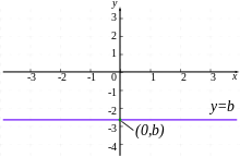
Horizontal Line y = b

This is a special case of the standard form where A = 0 and B = 1, or of the slope-intercept form where the slope m = 0. The graph is a horizontal line with y-intercept equal to b. There is no x-intercept, unless b = 0, in which case the graph of the line is the x-axis, and so every real number is an x-intercept.

x=a\,

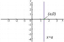
Vertical Line x = a

This is a special case of the standard form where A = 1 and B = 0. The graph is a vertical line with x-intercept equal to a. The slope is undefined. There is no y-intercept, unless a = 0, in which case the graph of the line is the y-axis, and so every real number is a y-intercept. This is the only type of straight line which is not the graph of a function (it obviously fails the vertical line test).

Connection with linear functions

A linear equation, written in the form y = f(x) whose graph crosses the origin (x,y) = (0,0), that is, whose y-intercept is 0, has the following properties:

f(x_{1}+x_{2})=f(x_{1})+f(x_{2})\

and

f(ax)=af(x),\,

where a is any scalar. A function which satisfies these properties is called a linear function (or linear operator, or more generally a linear map). However, linear equations that have non-zero y-intercepts, when written in this manner, produce functions which will have neither property above and hence are not linear functions in this sense. They are known as affine functions.

Examples

An everyday example of the use of different forms of linear equations is computation of tax with tax brackets. This is commonly done using either point–slope form or slope–intercept form; see Progressive tax#Computation for details.

More than two variables

A linear equation can involve more than two variables. Every linear equation in n unknowns may be rewritten

a_{1}x_{1}+a_{2}x_{2}+\cdots +a_{n}x_{n}=b,

where, a₁, a₂, ..., a_n represent numbers, called the coefficients, x₁, x₂, ..., x_n are the unknowns, and b is called the constant term. When dealing with three or fewer variables, it is common to use x, y and z instead of x₁, x₂ and x₃.

If all the coefficients are zero, then either b ≠ 0 and the equation does not have any solution, or b = 0 and every set of values for the unknowns is a solution.

If at least one coefficient is nonzero, a permutation of the subscripts allows to suppose a₁ ≠ 0, and rewrite the equation

x_{1}={\frac {b}{a_{1}}}-{\frac {a_{2}}{a_{1}}}x_{2}-\cdots -{\frac {a_{n}}{a_{1}}}x_{n}.

In other words, if a_i ≠ 0, one may choose arbitrary values for all the unknowns except x_i, and express x_i in term of these values.

If n = 3 the set of the solutions is a plane in a three-dimensional space. More generally, the set of the solutions is an (n – 1)-dimensional hyperplane in a n-dimensional Euclidean space (or affine space if the coefficients are complex numbers or belong to any field).

Notes

↑ Barnett, Ziegler & Byleen 2008, pg. 15

References

Barnett, R.A.; Ziegler, M.R.; Byleen, K.E. (2008), College Mathematics for Business, Economics, Life Sciences and the Social Sciences (11th ed.), Upper Saddle River, N.J.: Pearson, ISBN 0-13-157225-3

External links

Linear Equations and Inequalities Open Elementary Algebra textbook chapter on linear equations and inequalities.
Hazewinkel, Michiel, ed. (2001), "Linear equation", Encyclopedia of Mathematics, Springer, ISBN 978-1-55608-010-4

Polynomials and polynomial functions

By degree	Zero polynomial (degree undefined or −1 or −∞) Constant function (0) Linear function (1) Quadratic function (2) Cubic function (3) Quartic function (4) Quintic function (5) Sextic equation (6) Septic equation (7) Octic equation (8)

By number of terms and other properties	Monomial Binomial Trinomial Homogeneous Quasi-homogeneous

Tools and algorithms	Factorization Greatest common divisor Division Horner's method of evaluation Resultant Discriminant Gröbner basis

This article is issued from Wikipedia - version of the 11/14/2016. The text is available under the Creative Commons Attribution/Share Alike but additional terms may apply for the media files.