Kaplan–Meier estimator

An example of a Kaplan–Meier plot for two conditions associated with patient survival.

The Kaplan–Meier estimator,^[1][2] also known as the product limit estimator, is a non-parametric statistic used to estimate the survival function from lifetime data. In medical research, it is often used to measure the fraction of patients living for a certain amount of time after treatment. In other fields, Kaplan–Meier estimators may be used to measure the length of time people remain unemployed after a job loss,^[3] the time-to-failure of machine parts, or how long fleshy fruits remain on plants before they are removed by frugivores. The estimator is named after Edward L. Kaplan and Paul Meier, who each submitted similar manuscripts to the Journal of the American Statistical Association. The journal editor, John Tukey, convinced them to combine their work into one paper, which has been cited about 34,000 times since its publication.^[4]

Basic concepts

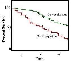
A plot of the Kaplan–Meier estimator is a series of declining horizontal steps which, with a large enough sample size, approaches the true survival function for that population. The value of the survival function between successive distinct sampled observations ("clicks") is assumed to be constant.

An important advantage of the Kaplan–Meier curve is that the method can take into account some types of censored data, particularly right-censoring, which occurs if a patient withdraws from a study, is lost to follow-up, or is alive without event occurrence at last follow-up. On the plot, small vertical tick-marks indicate individual patients whose survival times have been right-censored. When no truncation or censoring occurs, the Kaplan–Meier curve is the complement of the empirical distribution function.

In medical statistics, a typical application might involve grouping patients into categories, for instance, those with Gene A profile and those with Gene B profile. In the graph, patients with Gene B die much more quickly than those with gene A. After two years, about 80% of the Gene A patients survive, but less than half of patients with Gene B.

In order to generate a Kaplan–Meier estimator, at least two pieces of data are required for each patient (or each subject): the status at last observation (event occurrence or right-censored) and the time to event (or time to censoring). If the survival functions between two or more groups are to be compared, then a third piece of data is required: the group assignment of each subject.^[5]

Benefits and limitations

The Kaplan–Meier estimator is one of the most frequently used methods of survival analysis. The estimate may be useful to examine recovery rates, the probability of death, and the effectiveness of treatment. It is limited in its ability to estimate survival adjusted for covariates; parametric survival models and the Cox Proportional hazards model may be useful to estimate covariate-adjusted survival.

Example calculation of Kaplan-Meier estimate

The survival function S(t) is the probability that the lifetime of a member of a given population will be greater than the time t. The Kaplan–Meier estimator is a non-parametric estimator of the survival function. Hosmer and Lemeshow ^[6] describe the Kaplan–Meier estimator as follows. "This estimator incorporates information from all of the observations available, both uncensored and censored, by considering survival to any point in time as a series of steps defined by the observed survival and censored times. It is analogous to considering a toddler who must take five steps to walk from a chair to a table. This journey of five steps must begin with one successful step. The second step can only be taken if the first was successful. The third step can be taken only if the second (and also the first) was successful. Finally, the fifth step is possible only if the previous four were completed successfully. In an analysis of survival time, we estimated the conditional probabilities of "successful steps" and them multiply them together to obtain an estimate of the overall survivorship function."

Collett ^[7] describes the calculation of the Kaplan–Meier estimate as follows. "To obtain the Kaplan-Meier estimate, a series of time intervals is constructed … Each of these time intervals is designed to be such that one death time is contained in the interval, and this death time is take to occur at the start of the interval. As an illustration, suppose that t₍₁₎, t₍₂₎, and t₍₃₎ are three observed survival times arranged in rank order, so that t₍₁₎ < t₍₂₎ < t₍₃₎ and that c is a censored survival time that falls between t₍₂₎, and t₍₃₎. The constructed intervals than begin at times t₍₁₎, t₍₂₎, and t₍₃₎, and each interval includes one death time, although there could be more than one individual who dies at any particular time. Notice that no interval begins at the censored time of c. Now suppose that two individuals die at t₍₁₎, one dies at t₍₂₎, and and three die at t₍₃₎. The situation is illustrated diagrammatically in Figure 2.3 [the basis for the figure below], in which D represents a death and C a censored survival time."

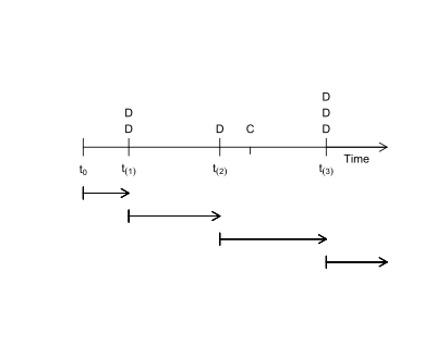
"The time origin is denoted by t0, and so there is an initial period commencing at t₀, which ends just before t₍₁₎, the time of the first death. This means that the interval from t₀ to t₍₁₎ will not include a death time. The first constructed interval extends from t1 to just before t2, and since the second death time is at t₍₂₎, this interval includes the single death time at t₍₁₎. The second interval begins at time t₍₂₎, and ends just before t₍₃₎, and includes the death time t₍₂₎ and the censored time c. There is also a third interval beginning at t₍₃₎, which contains the longest survival time, t₍₃₎." ^[7]

"In general, suppose that there are n individuals with observed survival times t₍₁₎, t₍₂₎, ..., t_(n). Some of these observations may be right censored, and there may also be more than one individual with the same observed survival time. We therefore suppose that there are r death times amongst the individuals, where r ≤ n. After arranging these death times in ascending order, the jth is denoted t_(j), for j = 1, 2, …, r, and so the r ordered death times are t₍₁₎ < t₍₂₎ < t_(r). The number of individuals who are alive just before time t_(j), including those who are about to die at this time, will be denoted n_(j), for j = 1, 2, …, r, and d_(j) will denote the number who die at this time…" ^[7]

"It sometimes happens that there are censored survival times that occur at the same time as one or more deaths, so that a death time and a censored survival time appear to occur simultaneously. In this situation, the censored time is taken to occur immediately after the death time when computing the value of [the number at risk] n_(j)." ^[7]

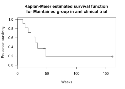
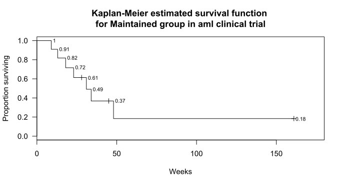
Tableman and Kim ^[8] give the following example. The data are time to relapse for acute myelogenous leukemia patients in a clinical trial. The data set aml is available in the R package "survival" and from the publisher's website (www.crcpress.com). For this example, only the 11 patients receiving extended treatment ("Maintained") are included. The weeks to relapse for the 11 patients were 9, 13, 13+, 18, 23, 28+, 31, 34, 45+, 48, and 161+ weeks, where the + sign indicates a censored observation. The Kaplan-Meier plot for these subjects is shown in the graph.

The Kaplan-Meier estimate for the aml data is constructed as follows. For the purpose of this example, the notation t_(j) for death times and d_(j) for number of deaths should be interpreted as relapse. The figure shows the time origin t₀ and the death times t₍₁₎, t₍₂₎, … , t₍₇₎. The death (relapse) times are indicated above the line, as are the times of censoring. The intervals t₍₁₎, t₍₂₎, … , t₍₇₎ are indicated below the line. Notice that each interval begins with a death. The censored observations at 28+, 45+, and 161+ weeks do not mark the beginning of an interval. The censored observation at 13+ weeks occurs at the same time as a death at 13 weeks, which marks the beginning of interval t₍₂₎. The number of censored observations in interval t_(j) is indicated by c_(j).

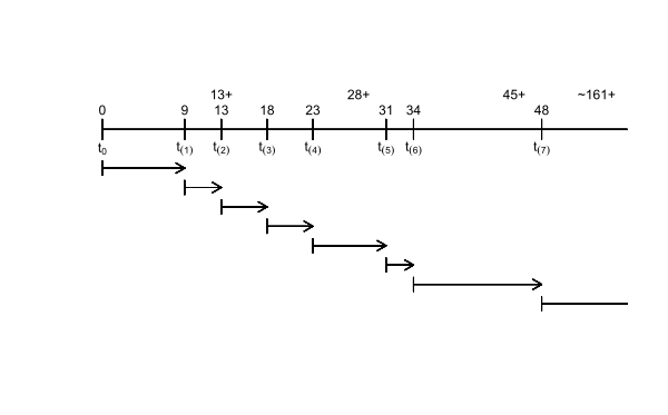
To calculate the Kaplan-Meier estimate, it is useful to lay out the aml data as shown in a table of ordered time intervals.^[9]

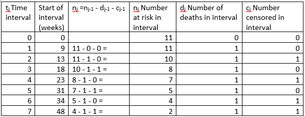
Column 1 in the table gives the ordered death times, t₍₁₎ to t₍₇₎, plus the time origin, t₀.

Column 2 gives the start of t_(j) in weeks.

Columns 3 and 4 show the number of subjects at risk at the start of the interval. The number at risk in the interval is n_(j) = n_(j-1) - d_(j-1) - c_(j-1), that is, the number at risk in the previous interval, minus losses due to death or censoring.

Column 5 is d_(j-1), the number of deaths in the interval.

Column 6 is c_(j-1), the number censored in the interval.

Time t₀

At the time origin t₀, all 11 subjects are alive, and the estimated probability of surviving past t₀ is 1.

${\displaystyle {\hat {S}}(t_{0})=1}$

Time t₍₁₎: 9 weeks

Next consider the time t₍₁₎ No deaths occur in the interval from t0 to just before t₍₁₎. No subjects are censored in the interval from t0 to just before t₍₁₎. At time t₍₁₎, n₍₁₎ = 11 patients are at risk d₍₁₎ = 1 patient dies

The probability of surviving past the t₍₁₎, given that the subject survived up to t₍₁₎, is therefore the proportion of the at-risk subjects who survive:

p₍₁₎ = (number at risk – number of deaths)/ (number at risk)

p₍₁₎ = (n₍₁₎ – d₍₁₎)/n₍₁₎ = (11 – 1)/11 = 0.91.

p₍₁₎ is called a conditional probability: it is conditional on the subject having survived up to t₍₁₎. For the aml data, the probability that the subject survived up to t₍₁₎ is the probability that they survived past t₀, which is :${\displaystyle {\hat {S}}(t_{0})=1}$

The Kaplan-Meier estimate of the probability that a subject will survive past time t1 is then

${\displaystyle {\hat {S}}(t_{1})={\hat {S}}(t_{0})*p_{1}=1*(11-1)/11=1*0.91=0.91}$

The first death time is at t₍₁₎ = 9 weeks. So the probability that a subject will survive past 9 weeks is

${\displaystyle {\hat {S}}(9)={\hat {S}}(t_{1})=0.91}$

Time t₍₂₎: 13 weeks

Next consider the time t₍₂₎ One death occurs in the interval from t₍₁₎ to just before t₍₂₎. No subjects are censored in the interval from t₍₁₎ to just before t₍₂₎. At time t₍₂₎, n₍₂₎ = 10 patients are at risk d₍₂₎ = 1 patient dies

The probability of surviving past the t₍₂₎, given that the subject survived up to t₍₂₎, is therefore the proportion

p₍₂₎ = (number at risk – number of deaths)/ (number at risk)

p₍₂₎ = (n₍₂₎ – d₍₂₎)/n₍₂₎ = (10 – 1)/10 = 0.9.

Again, p₍₂₎ is a conditional probability: it is conditional on the subject having survived up to t2. For the aml data, the probability that the subject survived up to t2 is the probability that they survived past t1, which was just calculated:

${\displaystyle {\hat {S}}(t_{1})=0.91}$

The Kaplan-Meier estimate of the probability that a subject will survive past time t₍₂₎ is then

${\displaystyle {\hat {S}}(t_{2})={\hat {S}}(t_{1})*p_{2}=0.91*0.9=0.818}$

Because ${\displaystyle {\hat {S}}(t_{1})={\hat {S}}(t_{0})*p_{1}}$, this equation can be re-written as

${\displaystyle {\hat {S}}(t_{2})={\hat {S}}(t_{0})*p_{1}*p_{2}=1*0.91*0.9=0.818}$

Further, because ${\displaystyle {\hat {S}}(t_{0})=1}$, the equation can be simplified to

${\displaystyle {\hat {S}}(t_{2})=p_{1}*p_{2}=0.91*0.9=0.818}$

The second death time is at t_2 = 13 weeks. So the probability that a subject will survive past 13 weeks is

${\displaystyle {\hat {S}}(13)={\hat {S}}(t_{2})=0.818}$

Time t₍₃₎: 18 weeks

Next consider time t₍₃₎. The calculation for time t₍₃₎, at week 18, requires accounting for the one subject who was censored at week 13. That subject is no longer in the risk set at week 18. As shown in the table of ordered time intervals above, the number at risk in the interval t_(j) is n_(j) = n_(j-1) - d_(j-1) - c_(j-1). For time t₍₃₎, this gives n₍₃₎ = n_(3-1) - d_(3-1) - c_(3-1). = 10 – 1 – 1 = 8 subjects at risk. Of the original 11 subjects, there are 2 deaths and 1 censored before t3, leaving the 8 at risk.

p₍₃₎ = (n₍₃₎ – d₍₃₎)/n₍₃₎ = (8– 1)/8= 0.875.

As before, p₍₃₎ is a conditional probability: it is conditional on the subject having survived up to t₍₃₎. The probability that the subject survived up to t₍₃₎ is the probability that they survived past t₍₂₎:

${\displaystyle {\hat {S}}(t_{2})=0.818}$

The Kaplan-Meier estimate of the probability that a subject will survive past time t₍₃₎ is then

${\displaystyle {\hat {S}}(t_{3})={\hat {S}}(t_{2})*p_{3}=0.818*0.875=0.716}$

Because ${\displaystyle {\hat {S}}(t_{2})=p_{1}*p_{2}=0.91*0.9=0.818}$, this equation can be re-written as

${\displaystyle {\hat {S}}(t_{3})=p_{1}*p_{2}*p_{3}=0.91*0.9*0.875=0.716}$

The third death time is at t₍₃₎ = 18 weeks. So the probability that a subject will survive past 18 weeks is

${\displaystyle {\hat {S}}(18)={\hat {S}}(t_{3})=0.716}$

Time t_(j): up to 161 weeks

The calculation of the Kaplan-Meier estimates ${\displaystyle {\hat {S}}(t_{j})}$ for all the times t₀ to t₍₇₎ are shown in the table.

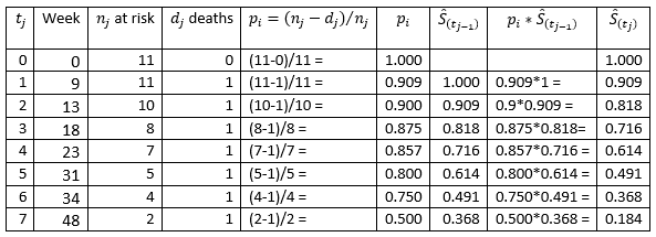
From these examples, it can be seen that the Kaplan-Meier estimate can be calculated as

${\displaystyle {\hat {S}}(t_{j})=p_{1}*p_{2}*\cdots *p_{j}}$

${\displaystyle {\hat {S}}(t)=\prod \limits _{t_{j}\leq t}{\frac {n_{j}-d_{j}}{n_{j}}}.}$

The table below summarizes the Kaplan-Meier estimates.

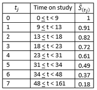
The graph shows the intervals and the Kaplan-Meier estimate of survival for each interval.

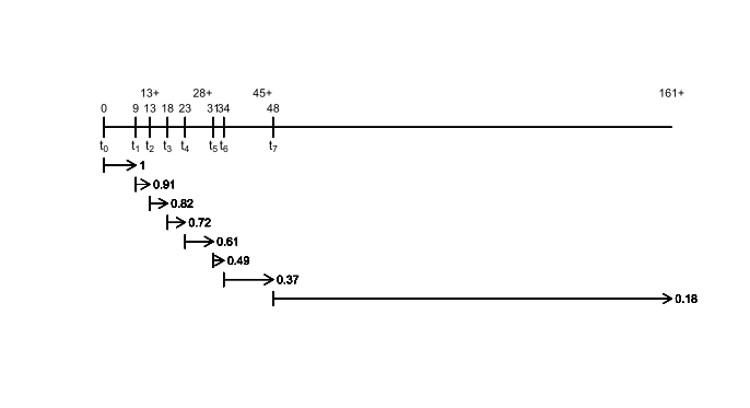
Finally, these estimates are displayed in a Kaplan-Meier plot as shown below, to which the estimate for each interval has been added. Censored subjects are indicated on the graph by a +, visible at weeks 28, 45, and 161.

When there is no censoring, n_j is simply the number of survivors just prior to time t_j. With censoring, n_j is the number of survivors minus the number of losses (censored cases). It is only those surviving cases that are still being observed (have not yet been censored) that are "at risk" of an (observed) death.^[10]

There is an alternative definition that is sometimes used, namely

${\displaystyle {\hat {S}}(t)=\prod \limits _{t_{j}<t}{\frac {n_{j}-d_{j}}{n_{j}}}.}$

The two definitions differ only at the observed event times. The first definition is right-continuous whereas the alternative definition is left-continuous.

Let T be the random variable that measures the time of failure and let F(t) be its cumulative distribution function. Note that

$S(t) = P[T>t] = 1-P[T \le t] = 1-F(t). \,$

Consequently, the right-continuous definition of $\scriptstyle\hat S(t)$ may be preferred in order to make the estimate compatible with a right-continuous estimate of F(t).

Statistical considerations

The Kaplan–Meier estimator is a statistic, and several estimators are used to approximate its variance. One of the most common such estimators is Greenwood's formula:^[11]

$\widehat {\operatorname {Var}}(\widehat S(t))=\widehat S(t)^{2}\sum \limits _{{t_{i}\leq t}}{\frac {d_{i}}{n_{i}(n_{i}-d_{i})}}.$

In some cases, one may wish to compare different Kaplan–Meier curves. This may be done by several methods including:

• The log rank test
• The Cox proportional hazards test

Other statistics that may be of use with this estimator are the Hall-Wellner band^[12] and the equal-precision band.^[13]

Implementations in statistics packages

• SAS: The Kaplan–Meier estimator is implemented in the proc lifetest procedure.^[14]
• R: the Kaplan–Meier estimator is available as part of the survival package.^[15][16][17]
• Stata: the command sts returns the Kaplan–Meier estimator.^[18][19]
• Python: the lifelines package includes the Kaplan–Meier estimator.^[20]
• MATLAB: the ecdf function with the 'function','survivor' arguments can calculate or plot the Kaplan–Meier estimator.^[21]

See also

• Frequency of exceedance
• Median lethal dose
• Nelson–Aalen estimator

References

1. Kaplan, E. L.; Meier, P. (1958). "Nonparametric estimation from incomplete observations". J. Amer. Statist. Assn. 53 (282): 457–481. doi:10.2307/2281868. JSTOR 2281868.
2. Kaplan, E.L. in a retrospective on the seminal paper in "This week's citation classic". Current Contents 24, 14 (1983). Available from UPenn as PDF.
3. Meyer, Bruce D. (1990). "Unemployment Insurance and Unemployment Spells". Econometrica. 58 (4): 757–782. doi:10.2307/2938349.
4. "Paul Meier, 1924–2011". Chicago Tribune. August 18, 2011.
5. Rich JT, Neely JG, Paniello RC, Voelker CC, Nussenbaum B, Wang EW (2010). "A practical guide to understanding Kaplan–Meier curves.". Otolaryngol Head Neck Surg. 143 (3): 331–6. doi:10.1016/j.otohns.2010.05.007. PMC 3932959. PMID 20723767.
6. Hosmer, David; Lemeshow, Stanley (1999), Applied Survival Analysis: Regression Modeling of Time to Event Data (First ed.), Wiley
7. Collett, David (2014), Modelling Survival Data in Medical Research (Third ed.), Chapman & Hall/CRC, ISBN 978-1439856789
8. Tableman, Mara; Kim, Jong Sung (2003), Survival Analysis Using S (First ed.), Chapman and Hall/CRC, ISBN 978-1584884088
9. Kleinbaum, David G.; Klein, Mitchel (2012), Survival analysis: A Self-learning text (Third ed.), Springer, ISBN 978-1441966452
10. Costella, John P. (2010). "A simple alternative to Kaplan–Meier for survival curves" (PDF). Unpublished.
11. Greenwood, M. (1926). "The natural duration of cancer". Reports on Public Health and Medical Subjects. London: Her Majesty's Stationery Office. 33: 1–26.
12. Hall WJ and Wellner JA (1980) Confidence bands for a survival curve for censored data. Biometrika 69
13. Nair VN (1984) Confidence bands for survival functions with censored data: A comparative study. Technometrics 26: 265–275
14. The LIFETEST Procedure
15. "survival: Survival Analysis". R Project.
16. Willekens, Frans (2014). "The Survival Package". Multistate Analysis of Life Histories with R. Springer. pp. 135–153. doi:10.1007/978-3-319-08383-4_6. ISBN 978-3-319-08383-4.
17. Chen, Ding-Geng; Peace, Karl E. (2014). Clinical Trial Data Analysis Using R. CRC Press. pp. 99–108.
18. "sts — Generate, graph, list, and test the survivor and cumulative hazard functions" (PDF). Stata Manual.
19. Cleves, Mario (2008). An Introduction to Survival Analysis Using Stata (Second ed.). College Station: Stata Press. pp. 93–107. ISBN 1-59718-041-6.
20. "lifelines"..
21. "Empirical cumulative distribution function - MATLAB ecdf". mathworks.com. Retrieved 2016-06-16.

Further reading

• Aalen, Odd; Borgan, Ornulf; Gjessing, Hakon (2008). Survival and Event History Analysis: A Process Point of View. Springer. pp. 90–104. ISBN 978-0-387-68560-1.
• Greene, William H. (2012). "Nonparametric and Semiparametric Approaches". Econometric Analysis (Seventh ed.). Prentice-Hall. pp. 909–912. ISBN 978-0-273-75356-8.
• Jones, Andrew M.; Rice, Nigel; D'Uva, Teresa Bago; Balia, Silvia (2013). "Duration Data". Applied Health Economics. London: Routledge. pp. 139–181. ISBN 978-0-415-67682-3.
• Singer, Judith B.; Willett, John B. (2003). Applied Longitudinal Data Analysis: Modeling Change and Event Occurrence. New York: Oxford University Press. pp. 483–487. ISBN 0-19-515296-4.

External links

• Calculating Kaplan–Meier curves by Steve Dunn
• Kaplan–Meier Survival Curves and the Log-Rank Test